Sentiment Analysis on Movie Reviews with PySS3
This is the notebook for the “Sentiment Analysis (on Movie Reviews)” tutorial. In this notebook, we will see how we can use the PySS3 Python package to deploy models for Sentiment Analysis on Movie Reviews.
Let us begin! First, we need to import the modules we will be using:
from pyss3 import SS3
from pyss3.util import Dataset, Evaluation, span
from pyss3.server import Live_Test

from sklearn.metrics import accuracy_score
… and unzip the “movie_review.zip” dataset inside the datasets folder.
!unzip -u datasets/movie_review.zip -d datasets/
Ok, now let’s create a new instance of the SS3 classifier.
clf = SS3()
What are the default hyperparameter values? let’s see
s, l, p, _ = clf.get_hyperparameters()

print("Smoothness(s):", s)
print("Significance(l):", l)
print("Sanction(p):", p)
Smoothness(s): 0.45
Significance(l): 0.5
Sanction(p): 1
Ok, now let’s load the training and the test set document files using
the load_from_files function from pyss3.util as follow:
x_train, y_train = Dataset.load_from_files("datasets/movie_review/train")
x_test, y_test = Dataset.load_from_files("datasets/movie_review/test")
[2/2] Loading 'pos' documents: 100%|██████████| 5000/5000 [00:00<00:00, 5649.90it/s]
[2/2] Loading 'pos' documents: 100%|██████████| 500/500 [00:00<00:00, 4703.76it/s]
Let’s train our model…
clf.train(x_train, y_train) # clf.fit(x_train, y_train)
Training on 'pos': 100%|██████████| 2/2 [00:13<00:00, 6.61s/it]
Note that we don’t have to create any document-term matrix! we are using
just the plain x_train documents :D cool uh? SS3 learns a (spacial
kind of) language model for each category and therefore it doesn’t need
to create any document-term matrices :) in fact, the very concept of
“document” becomes irrelevant…
Now that the model has been trained, let’s test it using the documents
in x_test. First, we will do it “in the sklearn’s own way” with:
y_pred = clf.predict(x_test)

accuracy = accuracy_score(y_pred, y_test)

print("Accuracy was:", accuracy)
Classification: 100%|██████████| 1000/1000 [00:03<00:00, 271.75it/s]

Accuracy was: 0.853
Alternatively, we could’ve done it “in the PySS3’s own way” by using the
built-in test function provided by the Evaluation class that we
have imported from pyss3.util at the beginning of this notebook, as
follows:
Evaluation.test(clf, x_test, y_test)
              precision    recall  f1-score   support

         neg       0.87      0.83      0.85       500
         pos       0.83      0.88      0.86       500

    accuracy                           0.85      1000
   macro avg       0.85      0.85      0.85      1000
weighted avg       0.85      0.85      0.85      1000
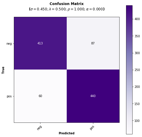
The advantage of using this built-in function is that with just a single line of code we get:
The performance measured in terms of all the well-known metrics (‘accuracy’, ‘precision’, ‘recall’, and ‘f1-score’).
A plot showing the obtained confusion matrix, and…
Since all the evaluations performed using the
Evaluationclass are permanently cached, if we ever perform this test again, the evaluation will be skipped and values will be retrieved from the cache storage (saving us a lot of time! when performing long evaluations).
As we can see, the performance doesn’t look bad using the default hyperparameter values, however, let’s now manually analyze what our model has actually learned by using the interactive “live test”.
Live_Test.run(clf, x_test, y_test)
Makes sense to you? (remember you can use the options to select “words” as the Description Level if you want to know based on what words, and to what degree, is making classification decisions)
Live test doesn’t look bad, however, we will create a “more intelligent”
model, a version of the model that can recognize variable-length word
n-grams “on the fly”. Thus, when calling the train we will pass an
extra argument n_grams=3 to indicate we want SS3 to learn to
recognize important words, bigrams, and 3-grams (If you’re curious and
want to know how this is actually done by SS3, read the paper “t-SS3: a
text classifier with dynamic n-grams for early risk detection over text
streams”, preprint available here ).
clf = SS3(name="reviews-3grams")

clf.train(x_train, y_train, n_grams=3)  # <-- note the n_grams=3 argument here
Training on 'pos': 100%|██████████| 2/2 [00:19<00:00, 10.00s/it]
Now let’s see if the performance has improved…
y_pred = clf.predict(x_test)
print("Accuracy:", accuracy_score(y_pred, y_test))
Classification: 100%|██████████| 1000/1000 [00:04<00:00, 243.31it/s]

Accuracy: 0.856
Yeah, the accuracy slightly improved but more importantly, we should now see that the model has learned “more intelligent patterns” involving sequences of words when using the interactive “live test” (like “was supposed to”, “has nothing to”, “low budget”, “your money”, etc. for the “negative” class). Let’s see…
Live_Test.run(clf, x_test, y_test)
If we want to improve performance even more, we could try using different hyperparameter values, for example, the following hyperparameter values will slightly improve our classification performance:
clf.set_hyperparameters(s=.44, l=.48, p=0.5)
Let’s see if it’s true…
y_pred = clf.predict(x_test)
print("Accuracy:", accuracy_score(y_pred, y_test))
Classification: 100%|██████████| 1000/1000 [00:05<00:00, 179.46it/s]

Accuracy: 0.861
Great! the accuracy has improved, indeed! :D
Finally, we could take a look at what our final model looks like using the Live Test tool one last time.
Live_Test.run(clf, x_test, y_test)
Want to know how we found out those hyperparameter values were going to improve our classifier accuracy? Just read the next section! ;)
Hyperparameter Optimization
In this section we will see how we can use PySS3’s Evaluation class
to perform Hyperparameter
optimization,
which allows us to find better hyperparameter values for our models. To
do this, we will perform grid
searches
using the
Evaluation.grid_search()
function.
Let’s create a new (standard) instance of the SS3 classifier. This will speed things up because the model we currently have in clf recognize variable-length word n-grams, the grid search won’t run as fast as with a (standard) model that recognize only words (and the same “best” hyperparameter values usually work for both of them).
Note
Just ignore the (optional) name argument below, we’re giving our model the name “movie-reviews” only to make things clearer when we create the interactive 3D evaluation plot.
clf = SS3(name="movie-reviews")

clf.train(x_train, y_train)
The
Evaluation.grid_search()
takes, for each hyperparameter, the list of values to use in the search,
for instance s=[0.25, 0.5, 0.75, 1] indicates you want the
grid_search to try out evaluating the classifier using those 4
values for the sigma (s) hyperparameter. However, for simplicity,
instead of using a manually crafted long list of values, we will use the
span function we have imported from pyss3.util at the beginning
of this notebook. This function will create a list of values for us,
giving a lower and upper bound, and the number of elements to be
generated. For instance, if we want a list of 6 numbers between 0 and 1,
we could use:
span(0, 1, 6)
[0. , 0.2, 0.4, 0.6, 0.8, 1. ]
Thus, we will use the following values for each of the three hyperparameters:
s_vals=span(0.2, 0.8, 6)  # [0.2 , 0.32, 0.44, 0.56, 0.68, 0.8]
l_vals=span(0.1, 2, 6)    # [0.1 , 0.48, 0.86, 1.24, 1.62, 2]
p_vals=span(0.5, 2, 6)    # [0.5, 0.8, 1.1, 1.4, 1.7, 2]
First, we will perform a grid search using the test set. Once the search
is over, Evaluation.grid_search will return the hyperparamter values
that obtained the best accuracy.
Note
Just ignore the tag argument below, do not worry about it,
it is optional. We are using it here just to give this search a name
("grid search (test)") because it will make identification of each
individual search clearer and easier for us in the last section
(“Interactive 3D Evaluation Plot”) when we need it.
# the search should take 2-3 minutes
best_s, best_l, best_p, _ = Evaluation.grid_search(
    clf, x_test, y_test,
    s=s_vals, l=l_vals, p=p_vals,
    tag="grid search (test)"  # <-- this is optional! >_<
)
Grid search: 100%|██████████| 216/216 [02:43<00:00, 4.75s/it]
print("The hyperparameter values that obtained the best Accuracy are:")
print("Smoothness(s):", best_s)
print("Significance(l):", best_l)
print("Sanction(p):", best_p)
The hyperparameter values that obtained the best Accuracy are:
Smoothness(s): 0.44
Significance(l): 0.48
Sanction(p): 0.5
And that’s how we found out that these hyperparameter values
(s=0.44, l=0.48, p=0.5) were going to improve our classifier
accuracy.
Finally, there is an optional (but recommended) step. To make sure the
selected hyperparameters generalize well (i.e. are not overfitted to the
test set), it is good practice to perform the grid search using k-fold
cross-validation on the training set. Thus, we’ll use the k_fold
argument of Evaluation.grid_search() to indicate we want to use
(stratified) 10-fold cross-validation (k_fold=10), as follows:
# the search should take 5-8 minutes
best_s, best_l, best_p, _ = Evaluation.grid_search(
    clf, x_train, y_train,
    k_fold=10,
    s=s_vals, l=l_vals, p=0.5,
    tag="grid search (10-fold)"  # <-- remember this is optional! >_<
)
[fold 10/10] Grid search: 100%|██████████| 36/36 [00:36<00:00, 4.78s/it]
print("The hyperparameter values that obtained the best accuracy are:")
print("Smoothness(s):", best_s)
print("Significance(l):", best_l)
print("Sanction(p):", best_p)
The hyperparameter values that obtained the best accuracy are:
Smoothness(s): 0.44
Significance(l): 0.48
Sanction(p): 0.5
The same hyperparameter values performed the best on the training data
using 10-fold cross-validation. This means we can use the selected
hyperparameter values (s=0.44, l=0.48 and p=0.5) safely.
Note that this time we used a fixed value for p, namely, p = 0.5
to perform the grid search. We decided to use this single value to speed
up the search since, as we will see in the next subsection, this
“sanction”(p) hyperparameter doesn’t seem to have a real impact on
performance in this task.
Note
What if we want to find hyperparameter values that performed
the best but using a different metric other than accuracy? for example,
what if we wanted to find the hyperparameter values that will improve
the precision for the (neg)ative class? we can use the
Evaluation.get_best_hyperparameters() function as follows:
s, l, p, _ = Evaluation.get_best_hyperparameters(metric="precision", metric_target="neg")

print("s=%.2f, l=%.2f, and p=%.2f" % (s, l, p))
s=0.56, l=2.0, and p=0.5
Or the macro averaged f1 score?
s, l, p, _ = Evaluation.get_best_hyperparameters(metric="f1-score", metric_target="macro avg")

print("s=%.2f, l=%.2f, and p=%.2f" % (s, l, p))
s=0.44, l=0.48, and p=0.5
Alternatively, we could have also added these 2 arguments, metric and
target, to the grid search in the first place :) (e.g. Evaluation.grid_search(..., metric="f1-score", metric_target="macro avg")).
Note that this get_best_hyperparameters function gave us the values
right away! this is because instead of performing the grid search again,
this function uses the evaluation cache to retrieve the best values from
disk, which save us a lot of time!
Interactive 3D Evaluation Plot
The Evaluation class comes with a really useful function,
Evaluation.plot(), that we can use to create an interactive 3D
evaluation plot (We highly recommend reading this brief
section,
from the documentation, in which it is briefly described). Instead of
using the single value returned from the Evaluation.grid_search() we
could use this plot to have a broader view of the relationship between
the different hyperparameter values and the performance of our model in
the task being addressed. The Evaluation.plot() function creates a
portable HTML file containing the interactive plot for us, and then
opens it up in your browser. Let’s give it a shot:
Evaluation.plot()
You should see a plot like this one:
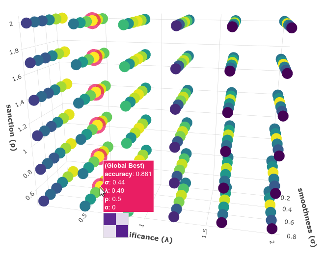
You probably noted that there are multiple points with the global best
performance, this is probably due to the problem being addressed
(sentiment analysis) being a binary classification problem (thus, the
“sanction” hyperparameter doesn’t have much impact with only two
categories). We could choose any of the best values, for instance,
grid_search gave us the one with the lowest “sanction” (p) value
(Rotate the plot and move the cursor over this point and see the
information that is displayed).
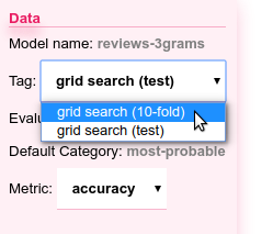
In the option panel (left side), note that in the “Tag” entry says “grid search (test)”, that means we are seeing evaluation results regarding the first grid search, the one we performed using the test set. To see the plot for the second grid search, in which we use 10-fold cross-validation, we can simply select its tag from the list:
In the plot for this second grid search not only can we see that the
same point (s=0.44, l=0.48, p=0.5) has the best performance, but
more importantly, if we move the cursor over this point, we can also see
that all the 10 confusion matrices looks really well and consistent,
that means that this hyperparameter configuration performed consistently
well across all 10 folds!
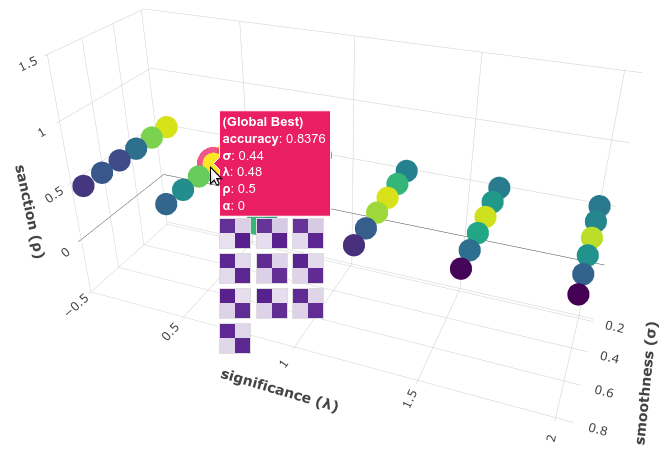
Therefore, we’re quite sure we can safely use the selected hyperparameter values :D
(Feel free to play a little bit with this interactive 3D evaluation plot, for instance try changing the metric and target from the options panel)