Topic Categorization
In this tutorial we will develop an SS3 classifier for topic categorization. We will work with a special dataset that we have created for this tutorial to train our model. This dataset was created collecting tweets with hashtags related to these 8 different categories: “art&photography”, “beauty&fashion”, “business&finance”, “food”, “health”, “music”, “science&technology” and “sports”. The dataset contains around 29k tweets for training on each category and only 100 tweets for testing on each one. Additionally, instead of having a folder for each category, training and test folder have a single .txt file for each category containing a tweet on each line. Finally, there’s an extra folder, called “live_test”, with 9 test documents that we will use to visually check that our model has learned properly. So, basically the dataset is structured like this:
datasets/topic
   ├── live_test
   │   └── test docs
   │       ├── doc_1.txt
   │       ├── doc_2.txt
   │       ├── doc_3.txt
   │       ├── doc_4.txt
   │       ├── doc_5.txt
   │       ├── doc_6.txt
   │       ├── doc_7.txt
   │       ├── doc_8.txt
   │       └── doc_9.txt
   ├── test
   │   ├── art&photography.txt
   │   ├── beauty&fashion.txt
   │   ├── business&finance.txt
   │   ├── food.txt
   │   ├── health.txt
   │   ├── music.txt
   │   ├── science&technology.txt
   │   └── sports.txt
   └── train
       ├── art&photography.txt
       ├── beauty&fashion.txt
       ├── business&finance.txt
       ├── food.txt
       ├── health.txt
       ├── music.txt
       ├── science&technology.txt
       └── sports.txt
Before we begin, go to Tutorial Setup and make sure you have everything we need.
As it is described in The Workflow, you can choose between two possible paths to carry out this tutorial: Classic Workflow (using python) or Command-Line Workflow (using only the PySS3 Command-Line tool)
Classic Workflow
Click here to go to the tutorial notebook.
Note
Want to run this Jupyter Notebook on your computer?
Go to Tutorial Setup and make sure you have everything we need.
Make sure you’re in the PySS3’s “examples” folder…
cd your/path/to/pyss3/examples
and that our conda environment is activated:
conda activate pyss3tutos
Then, lunch Jupyter Notebook and and run the “movie_review.ipynb” notebook (make sure to select the “pyss3tutos” kernel).
jupyter notebook
Command-Line Workflow
Note
Before beginning, make sure you have everything ready by reading the Tutorial Setup section.
Make sure you’re in the PySS3’s “examples” folder and that our conda environment is activated:
your@user:~$ cd /your/path/to/pyss3/examples
your@user:/your/path/to/pyss3/examples$ conda activate pyss3tutos
Make sure the dataset is unzipped, for instance by using unzip:
your@user:/your/path/to/pyss3/examples$ unzip -u datasets/topic.zip -d datasets/
Now use the “pyss3” command to run the PySS3 Command Line tool:
your@user:/your/path/to/pyss3/examples$ pyss3
We will create a new model using the new command, we will call this model “topic_categorization”:
(pyss3) >>> new topic_categorization
What are the default hyperparameter values? let’s see
(pyss3) >>> info
which displays the following:
NAME: topic_categorization


HYPERPARAMETERS:

   Smoothness(s): 0.45
   Significance(l): 0.5
   Sanction(p): 1

   Alpha(a): 0.0

CATEGORIES: None
That is, s=0.45, l=0.5, and p=1. Note that “CATEGORIES” is None which is OK since we haven’t trained our model yet.
To train train our model we will use the train command, let’s use the help command to see more details about this command:
(pyss3) >>> help train
which displays the following help:
Train the model using a training set and then save it.

usage:
    train TRAIN_PATH [LABEL] [N-gram]

required arguments:
 TRAIN_PATH     the training set path

optional arguments:
 LABEL          where to read category labels from.
                values:{file,folder} (default: folder)

 N-grams        indicates the maximum n-grams to be learned (e.g. a
                value of "1-grams" means only words will be learned;
                "2-grams" only 1-grams and 2-grams;
                "3-grams", only 1-grams, 2-grams and 3-grams;
                and so on).
                value: {N-grams} with N integer > 0 (default: 1-grams)

examples:
 train a/training/set/path 3-grams
train expects at least the path to the training set, and optionally, two extra arguments, LABEL and N-grams (we will ignore N-grams for now). LABEL takes two values, “file” or “folder”. Since there’s a single file for each category in our training set, we will use the argument “file” to tell PySS3 that each file is a different category and each line inside of it as a different document:
(pyss3) >>> train datasets/topic/train file
Now that the model has been trained, let’s see how good our model performs. To do this, since the test set has the same structure as the training set, we will use the test command also with the “file” extra argument:
(pyss3) >>> test datasets/topic/test file
which, among other things it displays:
accuracy: 0.704
Not bad using the default hyperparameter values, let’s now manually analyze what our model has actually learned by using the interactive “live test”.
(pyss3) >>> live_test datasets/topic/live_test
Note
here we are not using the “file” argument because inside the “live_test” folder each file is a different document (not a different category).
Live test doesn’t look bad, however, we will create a “more intelligent” version of this model, a version that can recognize variable-length word n-grams “on the fly”. So, let’s begin by creating a new model called “topic_categorization_3grams”:
(pyss3) >>> new topic_categorization_3grams
As we said above, we want this model to learn to recognize variable-length n-grams. Fortunately, as it was displayed with help train, we know that the train command accepts an extra argument: N-grams (where N is any positive integer). This argument will allow us to do what we want, we will use 3-grams to indicate we want SS3 to learn to recognize important words, bigrams, and 3-grams (*)
(pyss3) >>> train datasets/topic/train file 3-grams
(*) If you’re curious and want to know how this is actually done by SS3, read the paper “t-SS3: a ext classifier with dynamic n-grams for early risk detection over text streams” (preprint available here).
Now let’s see if the performance has improved…
(pyss3) >>> test datasets/topic/test file
which now displays:
accuracy: 0.719
Yeah, the accuracy slightly improved but more importantly, we should now see that the model has learned “more intelligent patterns” involving sequences of words when using the interactive “live test” to observe what our model has learned (like “machine learning”, “artificial intelligence”, “self-driving cars”, etc. for the “science&technology” category. Let’s see…
(pyss3) >>> live_test datasets/topic/live_test
Fortunately, our model has learned to recognize these important sequences (such as “artificial intelligence” and “machine learning” in doc_2.txt, “self-driving cars” in doc_6.txt, etc.). However, some documents aren’t perfectly classified, for instance, doc_3.txt was classified as “science&technology” (as a third topic) which is clearly wrong…
We will use better hyperparameter values to improve our classifier performance. Namely, we will set s=0.32, l=1.24 and p=1.1 which will improve the accuracy of our model:
(pyss3) >>> set s 0.32 l 1.24 p 1.1
Note
if you want to know how we found out that these values were going to improve our model’s accuracy, it is explained in the next subsection (Hyperparameter Optimization), so we really recommend reading it after completing this section.
Let’s see if the accuracy really improves using this values:
(pyss3) >>> test datasets/topic/test file
which displays:
accuracy: 0.771
Great! the accuracy improved :)
We will save this model in case we want to load it later…
(pyss3) >>> save
Optionally, you can again use the “live test” to manually check the final version of our model…
(pyss3) >>> live_test datasets/topic/live_test
Perfect! now the documents are classified properly! (including doc_3.txt) :D
And that’s it! use the following command to exit the PySS3 Command Line (or just press Ctrl+D):
(pyss3) >>> exit
Congratulations! you have created an SS3 model for topic categorization without a single line of code, buddy :)
Hyperparameter Optimization
As mentioned earlier, hyperparameter optimization will allow us to find better hyperparameter values for our model. To begin with, we will perform a grid search over the test set. To carry out this task, we will use the grid_search command. Let’s see what this command does and how to use it, using the help command:
(pyss3) >>> help grid_search
which displays the following help:
Given a dataset, perform a grid search using the given hyperparameters values.

usage:
    grid_search PATH [LABEL] [DEF_CAT] [METHOD] P EXP [P EXP ...] [no-cache]

required arguments:
 PATH       the dataset path
 P EXP      a list of values for a given hyperparameter.
            where:
             P    is a hyperparameter name. values: {s,l,p,a}
             EXP  is a python expression returning a float or
                  a list of floats. Note: if this expression
                  contains whitespaces, use quotations marks
                  (e.g. "[0.5, 1.5]")
            examples:
             s [.3,.4,.5]
             s "[.3, .4, .5]" (Note the whitespaces and the "")
             p r(.2,.8,6)     (i.e. 6 points between .2 to .8)

optional arguments:
 LABEL      where to read category labels from.
            values:{file,folder} (default: folder)

 DEF_CAT    default category to be assigned when the model is not
            able to actually classify a document.
            values: {most-probable,unknown} or a category label
            (default: most-probable)

 METHOD     the method to be used
            values: {test, K-fold} (default: test)
            where:
              K-fold  indicates the number of folds to be used.
                      K is an integer > 1 (e.g 4-fold, 10-fold, etc.)

 no-cache   if present, disable the cache and recompute all the values

examples:
 grid_search a/testset/path s r(.2,.8,6) l r(.1,2,6) -p r(.5,2,6) a [0,.01]
 grid_search a/dataset/path 4-fold -s [.2,.3,.4,.5] -l [.5,1,1.5] -p r(.5,2,6)
From this help, we can see that this command expects at least a path and a list of hyperparameter names and, after each hyperparameter name, any python expression that returns either a number or a list of numbers, for instance, -s [.2,.35,.4,.55]. In our case, we will use the built-in function r(x0,x1,n) which returns a list of n numbers between x0 and x1 (including both), as follows:
(pyss3) >>> grid_search datasets/topic/test file -s r(.2,.8,6) -l r(.1,2,6) -p r(.5,2,6)
Note that here, s will take 6 different values between .2 and .8, l between .1 and 2, and p between .5 and 2.
Now it is time to wait (for about 20 minutes) until the grid search is completed.
Once the grid search is over, we will use the following command to open up an interactive 3D plot in the browser that we can use to analyze the obtained results:
(pyss3) >>> plot evaluations
PySS3 should have created this plot on your machine. Note: We recommend reading the Interactive 3D Evaluation Plot page in which the plots and the user interface are explained in detail.
Rotate the plot and move the cursor over the point with the best performance (pink border) and see the information that is displayed, as shown in the following figure:
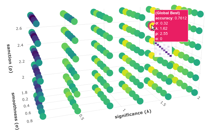
Here we can see that using these hyperparameter values, our classifier will obtain a better accuracy (0.7712):
smoothness (
 ): 0.32
significance (
 ): 1.24
sanction (
 ): 1.1
That is, we need to set s=0.32, l=1.24 and p=1.1. To do this we could use the set and save commands to update and save our model for later use:
(pyss3) >>> set s 0.32 l 1.24 p 1.1
(pyss3) >>> save
Note
if you want to use these hyperparameter values with python, there are at least three ways we can configure our SS3 classifier:
Creating a new classifier using these hyperparameter values:
clf = SS3(s=0.32, l=1.24, p=1.1)
Changing the hyperparameter values of an already existing model using the
set_hyperparametersmethod:
clf = SS3()
...
clf.set_hyperparameters(s=0.32, l=1.24, p=1.1)
Or, using the
PySS3 Command Line:Use the
setandsavecommands to update and save the model
(pyss3) >>> set s 0.32 l 1.24 p 1.1
(pyss3) >>> save
And then, use the
load_modelmethod to load the model with python:
clf = SS3(name="movie_review_3grams")
...
clf.load_model()